
En física , la teoría especial de la relatividad , o relatividad especial para abreviar, es una teoría científica de la relación entre el espacio y el tiempo . En el artículo de Albert Einstein de 1905, Sobre la electrodinámica de los cuerpos en movimiento , la teoría se presenta como basada en solo dos postulados : [p 1] [1] [2]
El primer postulado fue formulado por primera vez por Galileo Galilei (véase Invariancia galileana ).
La relatividad especial fue descrita por Albert Einstein en un artículo publicado el 26 de septiembre de 1905 titulado "Sobre la electrodinámica de los cuerpos en movimiento". [p 1] Las ecuaciones de Maxwell del electromagnetismo parecían ser incompatibles con la mecánica newtoniana , y el experimento de Michelson-Morley no logró detectar el movimiento de la Tierra frente al hipotético éter luminífero . Esto condujo al desarrollo de las transformaciones de Lorentz , por Hendrik Lorentz , que ajustan las distancias y los tiempos para los objetos en movimiento. La relatividad especial corrige las leyes de la mecánica hasta entonces vigentes para manejar situaciones que involucran todos los movimientos y especialmente aquellos a una velocidad cercana a la de la luz (conocida comovelocidades relativistas ). Hoy en día, se ha demostrado que la relatividad especial es el modelo más preciso del movimiento a cualquier velocidad cuando los efectos gravitacionales y cuánticos son insignificantes.[3][4]Aun así, el modelo newtoniano sigue siendo válido como una aproximación simple y precisa a bajas velocidades (relativas a la velocidad de la luz), por ejemplo, los movimientos cotidianos en la Tierra.
La relatividad especial tiene una amplia gama de consecuencias que han sido verificadas experimentalmente. [5] Incluyen la relatividad de la simultaneidad , la contracción de la longitud , la dilatación del tiempo , la fórmula relativista de adición de velocidad, el efecto Doppler relativista , la masa relativista , un límite de velocidad universal , la equivalencia masa-energía , la velocidad de causalidad y la precesión de Thomas . [1] [2] Por ejemplo, ha reemplazado la noción convencional de un tiempo universal absoluto con la noción de un tiempo que depende del marco de referencia y la posición espacial . En lugar de un intervalo de tiempo invariante entre dos eventos, hay un intervalo de espacio-tiempo invariante . Combinados con otras leyes de la física, los dos postulados de la relatividad especial predicen la equivalencia de masa y energía , como se expresa en la fórmula de equivalencia masa-energía , donde es la velocidad de la luz en el vacío. [6] [7] También explica cómo se relacionan los fenómenos de la electricidad y el magnetismo. [1] [2]
Una característica definitoria de la relatividad especial es la sustitución de las transformaciones galileanas de la mecánica newtoniana por las transformaciones de Lorentz . El tiempo y el espacio no pueden definirse por separado (como se creía anteriormente). Más bien, el espacio y el tiempo están entrelazados en un único continuo conocido como "espacio-tiempo" . Los acontecimientos que ocurren al mismo tiempo para un observador pueden ocurrir en momentos diferentes para otro.
Hasta varios años después, cuando Einstein desarrolló la relatividad general , que introdujo un espacio-tiempo curvado para incorporar la gravedad, no se utilizó la frase "relatividad especial". Una traducción que a veces se utiliza es "relatividad restringida"; "especial" en realidad significa "caso especial". [p 2] [p 3] [p 4] [nota 1] Parte del trabajo de Albert Einstein en relatividad especial se basa en el trabajo anterior de Hendrik Lorentz y Henri Poincaré . La teoría se completó esencialmente en 1907, con los artículos de Hermann Minkowski sobre el espacio-tiempo. [4]
La teoría es "especial" en el sentido de que sólo se aplica en el caso especial en el que el espacio-tiempo es "plano", es decir, donde la curvatura del espacio-tiempo (una consecuencia del tensor de energía-momento y que representa la gravedad ) es despreciable. [8] [nota 2] Para dar cabida correctamente a la gravedad, Einstein formuló la relatividad general en 1915. La relatividad especial, al contrario de algunas descripciones históricas, da cabida tanto a las aceleraciones como a los marcos de referencia acelerados . [9] [10]
Así como ahora se acepta que la relatividad galileana es una aproximación de la relatividad especial que es válida para velocidades bajas, la relatividad especial se considera una aproximación de la relatividad general que es válida para campos gravitatorios débiles , es decir, a una escala suficientemente pequeña (por ejemplo, cuando las fuerzas de marea son despreciables) y en condiciones de caída libre . Pero la relatividad general incorpora geometría no euclidiana para representar los efectos gravitatorios como la curvatura geométrica del espacio-tiempo. La relatividad especial está restringida al espacio-tiempo plano conocido como espacio de Minkowski . Mientras el universo pueda modelarse como una variedad pseudo-riemanniana , se puede definir un marco invariante de Lorentz que respete la relatividad especial para una vecindad suficientemente pequeña de cada punto en este espacio-tiempo curvado .
Galileo Galilei ya había postulado que no existe un estado de reposo absoluto y bien definido (no hay marcos de referencia privilegiados ), un principio que ahora se denomina principio de relatividad de Galileo . Einstein amplió este principio de modo que explicara la velocidad constante de la luz, [11] un fenómeno que se había observado en el experimento de Michelson-Morley. También postuló que se cumple para todas las leyes de la física , incluidas tanto las leyes de la mecánica como las de la electrodinámica . [12]
"Reflexiones de este tipo me hicieron comprender, ya poco después de 1900, es decir, poco después del trabajo pionero de Planck, que ni la mecánica ni la electrodinámica podían (salvo en casos limitados) reivindicar una validez exacta. Poco a poco fui perdiendo la esperanza de poder descubrir las leyes verdaderas mediante esfuerzos constructivos basados en hechos conocidos. Cuanto más lo intentaba y más desesperadamente, más llegaba a la convicción de que sólo el descubrimiento de un principio formal universal podía llevarnos a resultados seguros... ¿Cómo, entonces, podría encontrarse un principio tan universal?"
Albert Einstein: Notas autobiográficas [p 5]
Einstein distinguió dos proposiciones fundamentales que parecían ser las más seguras, independientemente de la validez exacta de las leyes (entonces) conocidas de la mecánica o la electrodinámica. Estas proposiciones eran la constancia de la velocidad de la luz en el vacío y la independencia de las leyes físicas (especialmente la constancia de la velocidad de la luz) de la elección del sistema inercial. En su presentación inicial de la relatividad especial en 1905, expresó estos postulados como: [p 1]
La constancia de la velocidad de la luz fue motivada por la teoría del electromagnetismo de Maxwell [13] y la falta de evidencia del éter luminífero . [14] Hay evidencia contradictoria sobre el grado en que Einstein fue influenciado por el resultado nulo del experimento de Michelson-Morley. [15] [16] En cualquier caso, el resultado nulo del experimento de Michelson-Morley ayudó a que la noción de la constancia de la velocidad de la luz ganara una aceptación generalizada y rápida.
La derivación de la relatividad especial depende no sólo de estos dos postulados explícitos, sino también de varias suposiciones tácitas ( hechas en casi todas las teorías de la física ), incluyendo la isotropía y homogeneidad del espacio y la independencia de las varas de medición y los relojes de su historia pasada. [p 6]
Tras la presentación original de la relatividad especial por parte de Einstein en 1905, se han propuesto muchos conjuntos diferentes de postulados en diversas derivaciones alternativas. [17] Pero el conjunto de postulados más común sigue siendo el empleado por Einstein en su artículo original. Una declaración más matemática del principio de relatividad hecha posteriormente por Einstein, que introduce el concepto de simplicidad no mencionado anteriormente, es:
Principio especial de relatividad : Si se elige un sistema de coordenadas K de modo que, en relación con él, las leyes físicas se cumplan en su forma más simple, las mismas leyes se cumplen en relación con cualquier otro sistema de coordenadas K ′ que se mueva en traslación uniforme con respecto a K . [18]
Henri Poincaré proporcionó el marco matemático para la teoría de la relatividad al demostrar que las transformaciones de Lorentz son un subconjunto de su grupo de Poincaré de transformaciones de simetría. Einstein derivó posteriormente estas transformaciones a partir de sus axiomas.
Muchos de los artículos de Einstein presentan derivaciones de la transformación de Lorentz basadas en estos dos principios. [p 7]
Los marcos de referencia desempeñan un papel crucial en la teoría de la relatividad. El término marco de referencia tal como se utiliza aquí es una perspectiva de observación en el espacio que no sufre ningún cambio de movimiento (aceleración), desde el que se puede medir una posición a lo largo de tres ejes espaciales (es decir, en reposo o a velocidad constante). Además, un marco de referencia tiene la capacidad de determinar mediciones del tiempo de los eventos utilizando un "reloj" (cualquier dispositivo de referencia con periodicidad uniforme).
Un evento es un suceso al que se le puede asignar un único momento y ubicación en el espacio en relación con un marco de referencia: es un "punto" en el espacio-tiempo . Dado que la velocidad de la luz es constante en relatividad independientemente del marco de referencia, los pulsos de luz se pueden utilizar para medir distancias de forma inequívoca y hacer referencia al reloj a los momentos en que ocurrieron los eventos, aunque la luz tarda en llegar al reloj después de que el evento haya ocurrido.
Por ejemplo, la explosión de un petardo puede considerarse un "acontecimiento". Podemos especificar completamente un acontecimiento mediante sus cuatro coordenadas espacio-temporales: el momento en que se produce y su ubicación espacial tridimensional definen un punto de referencia. Llamemos a este marco de referencia S .
En la teoría de la relatividad, a menudo queremos calcular las coordenadas de un evento a partir de diferentes sistemas de referencia. Las ecuaciones que relacionan las mediciones realizadas en diferentes sistemas se denominan ecuaciones de transformación .
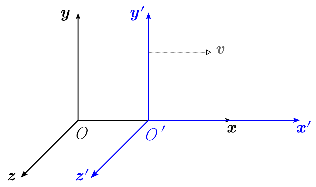
Para comprender mejor cómo se comparan entre sí las coordenadas del espacio-tiempo medidas por observadores en diferentes marcos de referencia , es útil trabajar con una configuración simplificada con marcos en una configuración estándar . [19] : 107 Con cuidado, esto permite simplificar las matemáticas sin pérdida de generalidad en las conclusiones a las que se llega. En la Fig. 2-1, se muestran dos marcos de referencia galileanos (es decir, marcos convencionales de 3 espacios) en movimiento relativo. El marco S pertenece a un primer observador O , y el marco S ′ (pronunciado "S prima" o "S guión") pertenece a un segundo observador O ′ .
Como no existe un sistema de referencia absoluto en la teoría de la relatividad, no existe estrictamente el concepto de "movimiento", ya que todo puede estar moviéndose con respecto a algún otro sistema de referencia. En cambio, se dice que dos sistemas cualesquiera que se muevan a la misma velocidad en la misma dirección están en co-movimiento . Por lo tanto, S y S ′ no están en co-movimiento .
El principio de relatividad , que establece que las leyes físicas tienen la misma forma en cada sistema de referencia inercial , se remonta a Galileo y fue incorporado a la física newtoniana. Pero a finales del siglo XIX, la existencia de ondas electromagnéticas llevó a algunos físicos a sugerir que el universo estaba lleno de una sustancia que llamaron " éter ", que, según postularon, actuaría como el medio a través del cual se propagarían estas ondas o vibraciones (en muchos aspectos de manera similar a la forma en que el sonido se propaga a través del aire). Se pensaba que el éter era un sistema de referencia absoluto contra el cual se podían medir todas las velocidades, y podía considerarse fijo e inmóvil en relación con la Tierra o algún otro punto de referencia fijo. Se suponía que el éter era lo suficientemente elástico como para soportar ondas electromagnéticas, mientras que esas ondas podían interactuar con la materia, pero no ofrecer resistencia a los cuerpos que pasaban a través de él (su única propiedad era que permitía que las ondas electromagnéticas se propagaran). Los resultados de varios experimentos, incluido el experimento de Michelson-Morley en 1887 (posteriormente verificado con experimentos más precisos e innovadores), condujeron a la teoría de la relatividad especial, al demostrar que el éter no existía. [20] La solución de Einstein fue descartar la noción de éter y el estado de reposo absoluto. En relatividad, cualquier sistema de referencia que se mueva con un movimiento uniforme observará las mismas leyes de la física. En particular, la velocidad de la luz en el vacío siempre se mide como c , incluso cuando se mide por múltiples sistemas que se mueven a velocidades diferentes (pero constantes).
A partir del principio de relatividad únicamente y sin asumir la constancia de la velocidad de la luz (es decir, utilizando la isotropía del espacio y la simetría implícita en el principio de relatividad especial), se puede demostrar que las transformaciones del espacio-tiempo entre sistemas inerciales son euclidianas, galileanas o lorentzianas. En el caso lorentziano, se puede obtener la conservación del intervalo relativista y una cierta velocidad límite finita. Los experimentos sugieren que esta velocidad es la velocidad de la luz en el vacío. [p 8] [21]
Einstein basó sistemáticamente la derivación de la invariancia de Lorentz (el núcleo esencial de la relatividad especial) únicamente en los dos principios básicos de la relatividad y la invariancia de la velocidad de la luz. Escribió:
La idea fundamental de la teoría especial de la relatividad es la siguiente: los supuestos de relatividad e invariancia de la velocidad de la luz son compatibles si se postulan relaciones de un nuevo tipo ("transformación de Lorentz") para la conversión de coordenadas y tiempos de eventos... El principio universal de la teoría especial de la relatividad está contenido en el postulado: las leyes de la física son invariantes con respecto a las transformaciones de Lorentz (para la transición de un sistema inercial a cualquier otro sistema inercial elegido arbitrariamente). Este es un principio restrictivo para las leyes naturales... [p 5]
Por ello, muchos tratamientos modernos de la relatividad especial la basan en el postulado único de la covariancia universal de Lorentz o, equivalentemente, en el postulado único del espacio-tiempo de Minkowski . [p 9] [p 10]
En lugar de considerar la covariancia universal de Lorentz como un principio derivado, este artículo la considera como el postulado fundamental de la relatividad especial. El enfoque tradicional de dos postulados para la relatividad especial se presenta en innumerables libros de texto universitarios y presentaciones populares. [22] Los libros de texto que comienzan con el postulado único del espacio-tiempo de Minkowski incluyen los de Taylor y Wheeler [11] y los de Callahan. [23] Este es también el enfoque seguido por los artículos de Wikipedia Espacio-tiempo y Diagrama de Minkowski .
Definamos un evento con coordenadas espaciotemporales ( t , x , y , z ) en el sistema S y ( t ′ , x ′ , y ′ , z ′ ) en un marco de referencia que se mueve a una velocidad v en el eje x con respecto a ese marco, S ′ . Luego, la transformación de Lorentz especifica que estas coordenadas están relacionadas de la siguiente manera: donde es el factor de Lorentz y c es la velocidad de la luz en el vacío, y la velocidad v de S ′ , relativa a S , es paralela al eje x . Para simplificar, las coordenadas y y z no se ven afectadas; solo se transforman las coordenadas x y t . Estas transformaciones de Lorentz forman un grupo de un parámetro de aplicaciones lineales , cuyo parámetro se denomina rapidez .
Resolviendo las cuatro ecuaciones de transformación anteriores para las coordenadas no primas se obtiene la transformación de Lorentz inversa:
Esto demuestra que el marco no preparado se mueve con la velocidad − v , medida en el marco preparado. [24]
El eje x no tiene nada de especial . La transformación se puede aplicar al eje y o al eje z , o incluso en cualquier dirección paralela al movimiento (que se deforma por el factor γ ) y perpendicular; consulte el artículo Transformación de Lorentz para obtener más detalles.
Una cantidad invariante bajo las transformaciones de Lorentz se conoce como escalar de Lorentz .
Escribiendo la transformación de Lorentz y su inversa en términos de diferencias de coordenadas, donde un evento tiene coordenadas ( x 1 , t 1 ) y ( x ′ 1 , t ′ 1 ) , otro evento tiene coordenadas ( x 2 , t 2 ) y ( x ′ 2 , t ′ 2 ) , y las diferencias se definen como
Nosotros conseguimos
Si tomamos diferenciales en lugar de tomar diferencias, obtenemos
Los diagramas de espacio-tiempo ( diagramas de Minkowski ) son una ayuda extremadamente útil para visualizar cómo se transforman las coordenadas entre diferentes sistemas de referencia. Aunque no es tan fácil realizar cálculos exactos utilizándolos como invocando directamente las transformaciones de Lorentz, su principal poder es su capacidad de proporcionar una comprensión intuitiva de los resultados de un escenario relativista. [21]
Para dibujar un diagrama de espacio-tiempo, comience por considerar dos marcos de referencia galileanos, S y S', en configuración estándar, como se muestra en la figura 2-1. [21] [25] : 155–199
Fig. 3-1a . Dibuje los ejes y del marco S. El eje es horizontal y el eje (en realidad ) es vertical, lo que es lo opuesto a la convención habitual en cinemática. El eje está escalado por un factor de de modo que ambos ejes tienen unidades de longitud comunes. En el diagrama mostrado, las líneas de cuadrícula están espaciadas una unidad de distancia. Las líneas diagonales de 45° representan las líneas de mundo de dos fotones que pasan por el origen en el tiempo La pendiente de estas líneas de mundo es 1 porque los fotones avanzan una unidad en el espacio por unidad de tiempo. Se han trazado dos eventos y en este gráfico de modo que sus coordenadas se puedan comparar en los marcos S y S'.
Fig. 3-1b . Dibuje los ejes y del marco S'. El eje representa la línea de mundo del origen del sistema de coordenadas S' medido en el marco S. En esta figura, los ejes y están inclinados con respecto a los ejes no primarios en un ángulo donde Los ejes primarios y no primarios comparten un origen común porque los marcos S y S' se habían configurado en la configuración estándar, de modo que cuando
Fig. 3-1c . Las unidades en los ejes con cebadores tienen una escala diferente a las unidades en los ejes sin cebadores. A partir de las transformaciones de Lorentz, observamos que las coordenadas de en el sistema de coordenadas con cebadores se transforman a en el sistema de coordenadas sin cebadores. Asimismo, las coordenadas de en el sistema de coordenadas con cebadores se transforman a en el sistema sin cebadores. Dibuje líneas de cuadrícula paralelas al eje a través de los puntos medidos en el marco sin cebadores, donde es un entero. Asimismo, dibuje líneas de cuadrícula paralelas al eje a través de los puntos medidos en el marco sin cebadores. Utilizando el teorema de Pitágoras, observamos que el espaciado entre unidades es igual a veces el espaciado entre unidades, medido en el marco S. Esta relación siempre es mayor que 1 y, en última instancia, se acerca al infinito como
Fig. 3-1d . Puesto que la velocidad de la luz es invariante, las líneas de mundo de dos fotones que pasan por el origen en el tiempo todavía se trazan como líneas diagonales de 45°. Las coordenadas primadas de y están relacionadas con las coordenadas no primadas a través de las transformaciones de Lorentz y podrían medirse aproximadamente a partir del gráfico (suponiendo que se haya trazado con la suficiente precisión), pero el verdadero mérito de un diagrama de Minkowski es que nos otorga una visión geométrica del escenario. Por ejemplo, en esta figura, observamos que los dos eventos separados en el tiempo que tenían diferentes coordenadas x en el marco no primado ahora están en la misma posición en el espacio.
Mientras que el marco sin primar está dibujado con ejes de espacio y tiempo que se encuentran en ángulos rectos, el marco primar está dibujado con ejes que se encuentran en ángulos agudos u obtusos. Esta asimetría se debe a distorsiones inevitables en la forma en que las coordenadas del espacio-tiempo se asignan a un plano cartesiano , pero los marcos son en realidad equivalentes.
Las consecuencias de la relatividad especial pueden derivarse de las ecuaciones de transformación de Lorentz . [26] Estas transformaciones, y por lo tanto la relatividad especial, conducen a predicciones físicas diferentes a las de la mecánica newtoniana en todas las velocidades relativas, y más pronunciadas cuando las velocidades relativas se vuelven comparables a la velocidad de la luz. La velocidad de la luz es mucho mayor que cualquier cosa que la mayoría de los humanos encuentren, por lo que algunos de los efectos predichos por la relatividad son inicialmente contraintuitivos .
En la relatividad galileana, la longitud de un objeto ( ) [nota 3] y la separación temporal entre dos eventos ( ) son invariantes independientes, cuyos valores no cambian cuando se observan desde diferentes marcos de referencia. [nota 4] [nota 5]
Sin embargo, en relatividad especial, el entrelazamiento de coordenadas espaciales y temporales genera el concepto de intervalo invariante , denotado como : [nota 6]
El entrelazamiento del espacio y el tiempo revoca los conceptos implícitos de simultaneidad absoluta y sincronización a través de marcos no comóviles.
La forma de ser la diferencia del cuadrado del lapso de tiempo y la distancia espacial al cuadrado, demuestra una discrepancia fundamental entre las distancias euclidianas y del espacio-tiempo. [nota 7] La invariancia de este intervalo es una propiedad de la transformada general de Lorentz (también llamada transformación de Poincaré ), lo que la convierte en una isometría del espacio-tiempo. La transformada general de Lorentz extiende la transformada de Lorentz estándar (que trata con traslaciones sin rotación, es decir, impulsos de Lorentz , en la dirección x) con todas las demás traslaciones , reflexiones y rotaciones entre cualquier marco inercial cartesiano. [30] : 33–34
En el análisis de escenarios simplificados, como los diagramas de espacio-tiempo, a menudo se emplea una forma de dimensionalidad reducida del intervalo invariante:
Demostrar que el intervalo es invariante es sencillo para el caso de dimensionalidad reducida y con marcos en configuración estándar: [21]
El valor de es por tanto independiente del marco en el que se mide.
Al considerar el significado físico de , hay tres casos a tener en cuenta: [21] [31] : 25–39

Consideremos dos eventos que suceden en dos lugares diferentes y que ocurren simultáneamente en el marco de referencia de un observador inercial. Pueden ocurrir de manera no simultánea en el marco de referencia de otro observador inercial (falta de simultaneidad absoluta ).
De la ecuación 3 (la transformación de Lorentz hacia adelante en términos de diferencias de coordenadas)
Es evidente que los dos eventos que son simultáneos en el marco S (satisfaciendo Δ t = 0 ), no son necesariamente simultáneos en otro marco inercial S ′ (satisfaciendo Δ t ′ = 0 ). Sólo si estos eventos son además co-locales en el marco S (satisfaciendo Δ x = 0 ), serán simultáneos en otro marco S ′ .
El efecto Sagnac puede considerarse una manifestación de la relatividad de la simultaneidad. [32] Dado que la relatividad de la simultaneidad es un efecto de primer orden en , [21] los instrumentos basados en el efecto Sagnac para su funcionamiento, como los giroscopios láser de anillo y los giroscopios de fibra óptica , son capaces de alcanzar niveles extremos de sensibilidad. [p 14]
El lapso de tiempo entre dos eventos no es invariable de un observador a otro, sino que depende de las velocidades relativas de los marcos de referencia de los observadores.
Supongamos que un reloj está en reposo en el sistema no primo S . La posición del reloj en dos tics diferentes se caracteriza entonces por Δ x = 0 . Para encontrar la relación entre los tiempos entre estos tics medidos en ambos sistemas, se puede utilizar la ecuación 3 para encontrar:
Esto demuestra que el tiempo (Δ t ′ ) entre los dos tics, como se ve en el marco en el que se mueve el reloj ( S ′ ), es más largo que el tiempo (Δ t ) entre estos tics, medido en el marco de reposo del reloj ( S ). La dilatación del tiempo explica una serie de fenómenos físicos; por ejemplo, la vida útil de los muones de alta velocidad creados por la colisión de rayos cósmicos con partículas en la atmósfera exterior de la Tierra y que se mueven hacia la superficie es mayor que la vida útil de los muones que se mueven lentamente, creados y decayendo en un laboratorio. [33]

Siempre que se oye una afirmación del tipo "los relojes en movimiento van más despacio", hay que imaginarse un sistema de referencia inercial poblado de relojes idénticos y sincronizados. A medida que un reloj en movimiento recorre este sistema, su lectura en cualquier punto concreto se compara con la de un reloj estacionario en el mismo punto. [34] : 149–152
Las mediciones que obtendríamos si miráramos un reloj en movimiento no serían, en general, en absoluto las mismas, porque el tiempo que veríamos estaría retrasado por la velocidad finita de la luz, es decir, los tiempos que vemos estarían distorsionados por el efecto Doppler . Las mediciones de los efectos relativistas siempre deben entenderse como realizadas después de que se hayan descartado los efectos de la velocidad finita de la luz. [34] : 149–152

Paul Langevin , uno de los primeros defensores de la teoría de la relatividad, hizo mucho por popularizar la teoría frente a la resistencia de muchos físicos a los conceptos revolucionarios de Einstein. Entre sus numerosas contribuciones a los fundamentos de la relatividad especial se encuentran trabajos independientes sobre la relación masa-energía, un examen exhaustivo de la paradoja de los gemelos e investigaciones sobre sistemas de coordenadas rotatorios. Su nombre se asocia con frecuencia a un concepto hipotético llamado "reloj de luz" (desarrollado originalmente por Lewis y Tolman en 1909 [35] ) que utilizó para realizar una novedosa derivación de la transformación de Lorentz. [36]
Se considera que un reloj de luz es una caja de paredes perfectamente reflectantes en la que una señal luminosa se refleja de un lado a otro desde caras opuestas. El concepto de dilatación del tiempo se enseña con frecuencia utilizando un reloj de luz que se desplaza en un movimiento inercial uniforme perpendicular a una línea que conecta los dos espejos. [37] [38] [39] [40] (El propio Langevin utilizó un reloj de luz orientado en paralelo a su línea de movimiento. [36] )
Consideremos el escenario ilustrado en la Fig. 4-3A. El observador A sostiene un reloj de luz de longitud así como un cronómetro electrónico con el que mide cuánto tarda un pulso en hacer un viaje de ida y vuelta a lo largo del reloj de luz. Aunque el observador A viaja rápidamente a lo largo de un tren, desde su punto de vista la emisión y recepción del pulso ocurren en el mismo lugar, y mide el intervalo utilizando un solo reloj ubicado en la posición precisa de estos dos eventos. Para el intervalo entre estos dos eventos, el observador A encuentra Un intervalo de tiempo medido utilizando un solo reloj que está inmóvil en un marco de referencia particular se llama intervalo de tiempo propio . [41]
La figura 4-3B ilustra estos mismos dos eventos desde el punto de vista del observador B, que está estacionado junto a las vías mientras el tren pasa a una velocidad de En lugar de hacer movimientos rectos hacia arriba y hacia abajo, el observador B ve los pulsos moviéndose a lo largo de una línea en zigzag. Sin embargo, debido al postulado de la constancia de la velocidad de la luz, la velocidad de los pulsos a lo largo de estas líneas diagonales es la misma que la que el observador A vio para sus pulsos hacia arriba y hacia abajo. B mide la velocidad del componente vertical de estos pulsos como de modo que el tiempo total de ida y vuelta de los pulsos es Nótese que para el observador B, la emisión y recepción del pulso de luz ocurrieron en diferentes lugares, y midió el intervalo utilizando dos relojes estacionarios y sincronizados ubicados en dos posiciones diferentes en su marco de referencia. El intervalo que B midió, por lo tanto, no fue un intervalo de tiempo propio porque no lo midió con un solo reloj en reposo. [41]
En la descripción anterior del reloj de luz de Langevin, la clasificación de un observador como estacionario y del otro como en movimiento fue completamente arbitraria. También podría suceder que el observador B llevara el reloj de luz y se moviera a una velocidad de hacia la izquierda, en cuyo caso el observador A percibiría que el reloj de B funcionaba más lento que su reloj local.
No hay ninguna paradoja aquí, porque no hay un observador independiente C que esté de acuerdo con A y B. El observador C necesariamente hace sus mediciones a partir de su propio marco de referencia. Si ese marco de referencia coincide con el marco de referencia de A, entonces C estará de acuerdo con la medición del tiempo de A. Si el marco de referencia de C coincide con el marco de referencia de B, entonces C estará de acuerdo con la medición del tiempo de B. Si el marco de referencia de C no coincide ni con el marco de A ni con el de B, entonces la medición del tiempo de C estará en desacuerdo con la medición del tiempo de A y de B. [42]
La reciprocidad de la dilatación del tiempo entre dos observadores en sistemas inerciales separados conduce a la llamada paradoja de los gemelos , articulada en su forma actual por Langevin en 1911. [43] Langevin imaginó a un aventurero que desea explorar el futuro de la Tierra. Este viajero se sube a un proyectil capaz de viajar al 99,995% de la velocidad de la luz. Después de hacer un viaje de ida y vuelta hacia y desde una estrella cercana que dura solo dos años de su propia vida, regresa a una Tierra que es doscientos años más vieja.
Este resultado parece desconcertante porque tanto el viajero como un observador terrestre verían al otro en movimiento y, por lo tanto, debido a la reciprocidad de la dilatación del tiempo, uno podría esperar inicialmente que cada uno de ellos hubiera encontrado que el otro había envejecido menos. En realidad, no hay ninguna paradoja, porque para que los dos observadores comparen sus tiempos propios, la simetría de la situación debe romperse: al menos uno de los dos observadores debe cambiar su estado de movimiento para que coincida con el del otro. [44]

Sin embargo, conocer la resolución general de la paradoja no permite calcular inmediatamente resultados cuantitativos correctos. En la literatura se han proporcionado muchas soluciones a este problema y se han analizado en el artículo sobre la paradoja de los gemelos . A continuación, examinaremos una de esas soluciones a la paradoja.
Nuestro objetivo básico será demostrar que, después del viaje, ambos gemelos están en perfecto acuerdo sobre quién envejeció cuánto, independientemente de sus diferentes experiencias. La figura 4-4 ilustra un escenario donde el gemelo viajero vuela a 0,6 c hacia y desde una estrella a 3 años luz de distancia. Durante el viaje, cada gemelo envía señales de tiempo anuales (medidas en sus propios tiempos propios) al otro. Después del viaje, se comparan los recuentos acumulativos. En la fase de ida del viaje, cada gemelo recibe las señales del otro a la tasa reducida de Inicialmente, la situación es perfectamente simétrica: observe que cada gemelo recibe la señal de un año del otro a los dos años medidos en su propio reloj. La simetría se rompe cuando el gemelo viajero se da la vuelta en la marca de los cuatro años medidos por su reloj. Durante los cuatro años restantes de su viaje, recibe señales a la tasa mejorada de La situación es bastante diferente con el gemelo estacionario. Debido al retraso de la velocidad de la luz, no ve a su hermana darse la vuelta hasta que hayan pasado ocho años en su propio reloj. Por lo tanto, recibe señales de frecuencia aumentada de su hermana durante un período relativamente breve. Aunque los gemelos no están de acuerdo en sus respectivas medidas del tiempo total, vemos en la siguiente tabla, así como por simple observación del diagrama de Minkowski, que cada gemelo está totalmente de acuerdo con el otro en cuanto al número total de señales enviadas de uno al otro. Por lo tanto, no hay ninguna paradoja. [34] : 152–159
Las dimensiones (por ejemplo, la longitud) de un objeto medidas por un observador pueden ser menores que los resultados de las mediciones del mismo objeto realizadas por otro observador (por ejemplo, la paradoja de la escalera implica una escalera larga que viaja casi a la velocidad de la luz y está contenida dentro de un garaje más pequeño).
De manera similar, supongamos que una varilla de medición está en reposo y alineada a lo largo del eje x en el sistema no primo S . En este sistema, la longitud de esta varilla se escribe como Δ x . Para medir la longitud de esta varilla en el sistema S ′ , en el que la varilla se está moviendo, las distancias x ′ a los puntos finales de la varilla deben medirse simultáneamente en ese sistema S ′ . En otras palabras, la medición se caracteriza por Δ t ′ = 0 , que se puede combinar con la Ecuación 4 para encontrar la relación entre las longitudes Δ x y Δ x ′ :
Esto demuestra que la longitud (Δ x ′ ) de la varilla medida en el marco en el que se mueve ( S ′ ), es más corta que su longitud (Δ x ) en su propio marco en reposo ( S ).
La dilatación del tiempo y la contracción de la longitud no son meras apariencias. La dilatación del tiempo está explícitamente relacionada con nuestra forma de medir los intervalos de tiempo entre eventos que ocurren en el mismo lugar en un sistema de coordenadas dado (llamados eventos "co-locales"). Estos intervalos de tiempo (que pueden ser, y son, medidos experimentalmente por observadores relevantes) son diferentes en otro sistema de coordenadas que se mueve con respecto al primero, a menos que los eventos, además de ser co-locales, también sean simultáneos. De manera similar, la contracción de la longitud se relaciona con nuestras distancias medidas entre eventos separados pero simultáneos en un sistema de coordenadas dado de elección. Si estos eventos no son co-locales, sino que están separados por la distancia (espacio), no ocurrirán a la misma distancia espacial entre sí cuando se los observe desde otro sistema de coordenadas en movimiento.
Consideremos dos marcos S y S ′ en configuración estándar. Una partícula en S se mueve en la dirección x con el vector de velocidad ¿Cuál es su velocidad en el marco S ′ ?
Podemos escribir
Sustituyendo expresiones para y de la ecuación 5 en la ecuación 8 , seguido de manipulaciones matemáticas sencillas y sustitución inversa de la ecuación 7, se obtiene la transformación de Lorentz de la velocidad en :
La relación inversa se obtiene intercambiando los símbolos primados y no primados y reemplazando con
Para no alineado a lo largo del eje x, escribimos: [12] : 47–49
Las transformaciones directa e inversa para este caso son:
La ecuación 10 y la ecuación 14 pueden interpretarse como la resultante de las dos velocidades y y reemplazan la fórmula que es válida en la relatividad galileana. Interpretadas de esa manera, se las conoce comúnmente como fórmulas relativistas de adición (o composición) de velocidades , válidas para los tres ejes de S y S ′ alineados entre sí (aunque no necesariamente en la configuración estándar). [12] : 47–49
Tomamos nota de los siguientes puntos:
No hay nada especial en la dirección x en la configuración estándar. El formalismo anterior se aplica a cualquier dirección; y tres direcciones ortogonales permiten tratar con todas las direcciones en el espacio descomponiendo los vectores de velocidad en sus componentes en estas direcciones. Consulte la fórmula de adición de velocidad para obtener más detalles.
La composición de dos impulsos de Lorentz no colineales (es decir, dos transformaciones de Lorentz no colineales, ninguna de las cuales implica rotación) da como resultado una transformación de Lorentz que no es un impulso puro, sino que es la composición de un impulso y una rotación.
La rotación de Thomas resulta de la relatividad de la simultaneidad. En la figura 4-5a, una varilla de longitud en su sistema de referencia en reposo (es decir, que tiene una longitud propia de ) se eleva verticalmente a lo largo del eje y en el sistema de referencia en el suelo.
En la figura 4-5b, se observa la misma varilla desde el marco de un cohete que se mueve a gran velocidad hacia la derecha. Si imaginamos dos relojes situados en los extremos izquierdo y derecho de la varilla que están sincronizados en el marco de la varilla , la relatividad de la simultaneidad hace que el observador en el marco del cohete observe (no vea) el reloj en el extremo derecho de la varilla como si estuviera adelantado en el tiempo y la varilla se observe correspondientemente como inclinada. [31] : 98–99
A diferencia de los efectos relativistas de segundo orden, como la contracción de la longitud o la dilatación del tiempo, este efecto se vuelve bastante significativo incluso a velocidades bastante bajas. Por ejemplo, esto se puede ver en el espín de partículas en movimiento , donde la precesión de Thomas es una corrección relativista que se aplica al espín de una partícula elemental o la rotación de un giroscopio macroscópico , relacionando la velocidad angular del espín de una partícula que sigue una órbita curvilínea con la velocidad angular del movimiento orbital. [31] : 169–174
La rotación de Thomas proporciona la solución a la conocida "paradoja del metro y el agujero". [p 15] [31] : 98–99

En la figura 4-6, el intervalo de tiempo entre los eventos A (la "causa") y B (el "efecto") es "temporal"; es decir, hay un marco de referencia en el que los eventos A y B ocurren en el mismo lugar en el espacio , separados solo por ocurrir en diferentes momentos. Si A precede a B en ese marco, entonces A precede a B en todos los marcos accesibles por una transformación de Lorentz. Es posible que la materia (o información) viaje (por debajo de la velocidad de la luz) desde el lugar de A, comenzando en el momento de A, hasta el lugar de B, llegando al momento de B, por lo que puede haber una relación causal (siendo A la causa y B el efecto).
El intervalo AC del diagrama es "similar al espacio", es decir, hay un marco de referencia en el que los eventos A y C ocurren simultáneamente, separados solo en el espacio. También hay marcos en los que A precede a C (como se muestra) y marcos en los que C precede a A. Pero no hay marcos accesibles mediante una transformación de Lorentz, en la que los eventos A y C ocurren en el mismo lugar. Si fuera posible que existiera una relación de causa y efecto entre los eventos A y C, se producirían paradojas de causalidad.
Por ejemplo, si las señales pudieran enviarse más rápido que la luz, entonces podrían enviarse señales al pasado del remitente (el observador B en los diagramas). [45] [p 16] Se podrían construir entonces diversas paradojas causales.
Considere los diagramas de espacio-tiempo de la figura 4-7. A y B se encuentran junto a una vía férrea cuando pasa un tren de alta velocidad, con C viajando en el último vagón del tren y D viajando en el vagón delantero. Las líneas de universo de A y B son verticales ( ct ), lo que distingue la posición estacionaria de estos observadores en el suelo, mientras que las líneas de universo de C y D están inclinadas hacia delante ( ct ′ ), lo que refleja el movimiento rápido de los observadores C y D estacionarios en su tren, tal como se observa desde el suelo.
No es necesario que las señales sean instantáneas para violar la causalidad. Incluso si la señal de D a C fuera ligeramente más superficial que el eje (y la señal de A a B ligeramente más inclinada que el eje), aún sería posible que B recibiera su mensaje antes de haberlo enviado. Al aumentar la velocidad del tren a velocidades cercanas a la de la luz, los ejes y pueden comprimirse muy cerca de la línea discontinua que representa la velocidad de la luz. Con esta configuración modificada, se puede demostrar que incluso señales solo ligeramente más rápidas que la velocidad de la luz darán como resultado una violación de la causalidad. [47]
Por lo tanto, si se quiere preservar la causalidad , una de las consecuencias de la relatividad especial es que ninguna señal de información ni ningún objeto material puede viajar más rápido que la luz en el vacío.
Esto no quiere decir que todas las velocidades superiores a la de la luz sean imposibles. Se pueden describir varias situaciones triviales en las que algunas "cosas" (no materia ni energía reales) se mueven más rápido que la luz. [48] Por ejemplo, el lugar donde el haz de luz de un reflector incide en la parte inferior de una nube puede moverse más rápido que la luz cuando el reflector se gira rápidamente (aunque esto no viola la causalidad ni ningún otro fenómeno relativista). [49] [50]

En 1850, Hippolyte Fizeau y Léon Foucault establecieron de forma independiente que la luz viaja más lentamente en el agua que en el aire, validando así una predicción de la teoría ondulatoria de la luz de Fresnel e invalidando la predicción correspondiente de la teoría corpuscular de Newton . [51] La velocidad de la luz se midió en agua en calma. ¿Cuál sería la velocidad de la luz en agua en movimiento?
En 1851, Fizeau realizó un experimento para responder a esta pregunta, cuya representación simplificada se ilustra en la figura 5-1. Un divisor de haz divide un haz de luz y los haces divididos pasan en direcciones opuestas a través de un tubo de agua en movimiento. Se recombinan para formar franjas de interferencia, que indican una diferencia en la longitud del recorrido óptico, que un observador puede ver. El experimento demostró que el arrastre de la luz por el agua en movimiento provocó un desplazamiento de las franjas, lo que demuestra que el movimiento del agua había afectado a la velocidad de la luz.
Según las teorías que prevalecían en ese momento, la luz que viaja a través de un medio en movimiento sería una simple suma de su velocidad a través del medio más la velocidad del medio. Contrariamente a lo esperado, Fizeau descubrió que, aunque la luz parecía ser arrastrada por el agua, la magnitud del arrastre era mucho menor de lo esperado. Si es la velocidad de la luz en agua quieta, y es la velocidad del agua, y es la velocidad de la luz transportada por el agua en el marco de referencia del laboratorio con el flujo de agua sumando o restando a la velocidad de la luz, entonces
Los resultados de Fizeau, aunque consistentes con la hipótesis anterior de Fresnel sobre el arrastre parcial del éter , fueron extremadamente desconcertantes para los físicos de la época. Entre otras cosas, la presencia de un término de índice de refracción significaba que, dado que depende de la longitud de onda, el éter debe ser capaz de sostener diferentes movimientos al mismo tiempo . [nota 8] Se propusieron diversas explicaciones teóricas para explicar el coeficiente de arrastre de Fresnel , que eran completamente contradictorias entre sí. Incluso antes del experimento de Michelson-Morley, los resultados experimentales de Fizeau se encontraban entre una serie de observaciones que crearon una situación crítica para explicar la óptica de los cuerpos en movimiento. [52]
Desde el punto de vista de la relatividad especial, el resultado de Fizeau no es más que una aproximación a la ecuación 10 , la fórmula relativista para la composición de velocidades. [30]

Debido a la velocidad finita de la luz, si los movimientos relativos de una fuente y un receptor incluyen un componente transversal, entonces la dirección desde la cual la luz llega al receptor se desplazará con respecto a la posición geométrica en el espacio de la fuente con respecto al receptor. El cálculo clásico del desplazamiento adopta dos formas y realiza predicciones diferentes dependiendo de si el receptor, la fuente o ambos están en movimiento con respecto al medio. (1) Si el receptor está en movimiento, el desplazamiento sería consecuencia de la aberración de la luz . El ángulo de incidencia del haz con respecto al receptor se podría calcular a partir de la suma vectorial de los movimientos del receptor y la velocidad de la luz incidente. [53] (2) Si la fuente está en movimiento, el desplazamiento sería consecuencia de la corrección del tiempo de luz . El desplazamiento de la posición aparente de la fuente con respecto a su posición geométrica sería el resultado del movimiento de la fuente durante el tiempo que tarda su luz en llegar al receptor. [54]
La explicación clásica no superó la prueba experimental. Dado que el ángulo de aberración depende de la relación entre la velocidad del receptor y la velocidad de la luz incidente, el paso de la luz incidente a través de un medio refractivo debería cambiar el ángulo de aberración. En 1810, Arago utilizó este fenómeno esperado en un intento fallido de medir la velocidad de la luz, [55] y en 1870, George Airy probó la hipótesis utilizando un telescopio lleno de agua, encontrando que, contra lo esperado, la aberración medida era idéntica a la aberración medida con un telescopio lleno de aire. [56] Un intento "engorroso" de explicar estos resultados utilizó la hipótesis del arrastre parcial del éter, [57] pero era incompatible con los resultados del experimento de Michelson-Morley, que aparentemente exigía un arrastre completo del éter. [58]
Suponiendo sistemas inerciales, la expresión relativista para la aberración de la luz es aplicable tanto a los casos de receptor en movimiento como a los de fuente en movimiento. Se han publicado diversas fórmulas trigonométricamente equivalentes. Expresadas en términos de las variables de la figura 5-2, estas incluyen [30] : 57–60
El efecto Doppler clásico depende de si la fuente, el receptor o ambos están en movimiento con respecto al medio. El efecto Doppler relativista es independiente de cualquier medio. Sin embargo, el efecto Doppler relativista para el caso longitudinal, con la fuente y el receptor moviéndose directamente uno hacia el otro o alejándose uno del otro, se puede derivar como si fuera el fenómeno clásico, pero modificado mediante la adición de un término de dilatación del tiempo , y ese es el tratamiento que se describe aquí. [59] [60]
Suponga que el receptor y la fuente se alejan entre sí con una velocidad relativa medida por un observador en el receptor o la fuente (la convención de signos adoptada aquí es que es negativa si el receptor y la fuente se mueven uno hacia el otro). Suponga que la fuente está estacionaria en el medio. Entonces, ¿dónde es la velocidad del sonido?
En el caso de la luz, y con el receptor moviéndose a velocidades relativistas, los relojes del receptor están dilatados en el tiempo en relación con los relojes de la fuente. El receptor medirá la frecuencia recibida para que esté donde
Se obtiene una expresión idéntica para el desplazamiento Doppler relativista cuando se realiza el análisis en el marco de referencia del receptor con una fuente en movimiento. [61] [21]
The transverse Doppler effect is one of the main novel predictions of the special theory of relativity.
Classically, one might expect that if source and receiver are moving transversely with respect to each other with no longitudinal component to their relative motions, that there should be no Doppler shift in the light arriving at the receiver.
Special relativity predicts otherwise. Fig. 5-3 illustrates two common variants of this scenario. Both variants can be analyzed using simple time dilation arguments.[21] In Fig. 5-3a, the receiver observes light from the source as being blueshifted by a factor of . In Fig. 5-3b, the light is redshifted by the same factor.

Time dilation and length contraction are not optical illusions, but genuine effects. Measurements of these effects are not an artifact of Doppler shift, nor are they the result of neglecting to take into account the time it takes light to travel from an event to an observer.
Scientists make a fundamental distinction between measurement or observation on the one hand, versus visual appearance, or what one sees. The measured shape of an object is a hypothetical snapshot of all of the object's points as they exist at a single moment in time. But the visual appearance of an object is affected by the varying lengths of time that light takes to travel from different points on the object to one's eye.

For many years, the distinction between the two had not been generally appreciated, and it had generally been thought that a length contracted object passing by an observer would in fact actually be seen as length contracted. In 1959, James Terrell and Roger Penrose independently pointed out that differential time lag effects in signals reaching the observer from the different parts of a moving object result in a fast moving object's visual appearance being quite different from its measured shape. For example, a receding object would appear contracted, an approaching object would appear elongated, and a passing object would have a skew appearance that has been likened to a rotation.[p 19][p 20][62][63] A sphere in motion retains the circular outline for all speeds, for any distance, and for all view angles, although the surface of the sphere and the images on it will appear distorted.[64][65]
.jpg/1280px-M87_jet_(1).jpg)
Both Fig. 5-4 and Fig. 5-5 illustrate objects moving transversely to the line of sight. In Fig. 5-4, a cube is viewed from a distance of four times the length of its sides. At high speeds, the sides of the cube that are perpendicular to the direction of motion appear hyperbolic in shape. The cube is actually not rotated. Rather, light from the rear of the cube takes longer to reach one's eyes compared with light from the front, during which time the cube has moved to the right. At high speeds, the sphere in Fig. 5-5 takes on the appearance of a flattened disk tilted up to 45° from the line of sight. If the objects' motions are not strictly transverse but instead include a longitudinal component, exaggerated distortions in perspective may be seen.[66] This illusion has come to be known as Terrell rotation or the Terrell–Penrose effect.[note 9]
Another example where visual appearance is at odds with measurement comes from the observation of apparent superluminal motion in various radio galaxies, BL Lac objects, quasars, and other astronomical objects that eject relativistic-speed jets of matter at narrow angles with respect to the viewer. An apparent optical illusion results giving the appearance of faster than light travel.[67][68][69] In Fig. 5-6, galaxy M87 streams out a high-speed jet of subatomic particles almost directly towards us, but Penrose–Terrell rotation causes the jet to appear to be moving laterally in the same manner that the appearance of the cube in Fig. 5-4 has been stretched out.[70]
Section Consequences derived from the Lorentz transformation dealt strictly with kinematics, the study of the motion of points, bodies, and systems of bodies without considering the forces that caused the motion. This section discusses masses, forces, energy and so forth, and as such requires consideration of physical effects beyond those encompassed by the Lorentz transformation itself.
As an object's speed approaches the speed of light from an observer's point of view, its relativistic mass increases thereby making it more and more difficult to accelerate it from within the observer's frame of reference.
The energy content of an object at rest with mass m equals mc2. Conservation of energy implies that, in any reaction, a decrease of the sum of the masses of particles must be accompanied by an increase in kinetic energies of the particles after the reaction. Similarly, the mass of an object can be increased by taking in kinetic energies.
In addition to the papers referenced above—which give derivations of the Lorentz transformation and describe the foundations of special relativity—Einstein also wrote at least four papers giving heuristic arguments for the equivalence (and transmutability) of mass and energy, for E = mc2.
Mass–energy equivalence is a consequence of special relativity. The energy and momentum, which are separate in Newtonian mechanics, form a four-vector in relativity, and this relates the time component (the energy) to the space components (the momentum) in a non-trivial way. For an object at rest, the energy–momentum four-vector is (E/c, 0, 0, 0): it has a time component which is the energy, and three space components which are zero. By changing frames with a Lorentz transformation in the x direction with a small value of the velocity v, the energy momentum four-vector becomes (E/c, Ev/c2, 0, 0). The momentum is equal to the energy multiplied by the velocity divided by c2. As such, the Newtonian mass of an object, which is the ratio of the momentum to the velocity for slow velocities, is equal to E/c2.
The energy and momentum are properties of matter and radiation, and it is impossible to deduce that they form a four-vector just from the two basic postulates of special relativity by themselves, because these do not talk about matter or radiation, they only talk about space and time. The derivation therefore requires some additional physical reasoning. In his 1905 paper, Einstein used the additional principles that Newtonian mechanics should hold for slow velocities, so that there is one energy scalar and one three-vector momentum at slow velocities, and that the conservation law for energy and momentum is exactly true in relativity. Furthermore, he assumed that the energy of light is transformed by the same Doppler-shift factor as its frequency, which he had previously shown to be true based on Maxwell's equations.[p 1] The first of Einstein's papers on this subject was "Does the Inertia of a Body Depend upon its Energy Content?" in 1905.[p 21] Although Einstein's argument in this paper is nearly universally accepted by physicists as correct, even self-evident, many authors over the years have suggested that it is wrong.[71] Other authors suggest that the argument was merely inconclusive because it relied on some implicit assumptions.[72]
Einstein acknowledged the controversy over his derivation in his 1907 survey paper on special relativity. There he notes that it is problematic to rely on Maxwell's equations for the heuristic mass–energy argument. The argument in his 1905 paper can be carried out with the emission of any massless particles, but the Maxwell equations are implicitly used to make it obvious that the emission of light in particular can be achieved only by doing work. To emit electromagnetic waves, all you have to do is shake a charged particle, and this is clearly doing work, so that the emission is of energy.[p 22][note 10]
In his fourth of his 1905 Annus mirabilis papers,[p 21] Einstein presented a heuristic argument for the equivalence of mass and energy. Although, as discussed above, subsequent scholarship has established that his arguments fell short of a broadly definitive proof, the conclusions that he reached in this paper have stood the test of time.
Einstein took as starting assumptions his recently discovered formula for relativistic Doppler shift, the laws of conservation of energy and conservation of momentum, and the relationship between the frequency of light and its energy as implied by Maxwell's equations.
Fig. 6-1 (top). Consider a system of plane waves of light having frequency traveling in direction relative to the x-axis of reference frame S. The frequency (and hence energy) of the waves as measured in frame S′ that is moving along the x-axis at velocity is given by the relativistic Doppler shift formula which Einstein had developed in his 1905 paper on special relativity:[p 1]
Fig. 6-1 (bottom). Consider an arbitrary body that is stationary in reference frame S. Let this body emit a pair of equal-energy light-pulses in opposite directions at angle with respect to the x-axis. Each pulse has energy . Because of conservation of momentum, the body remains stationary in S after emission of the two pulses. Let be the energy of the body before emission of the two pulses and after their emission.
Next, consider the same system observed from frame S′ that is moving along the x-axis at speed relative to frame S. In this frame, light from the forwards and reverse pulses will be relativistically Doppler-shifted. Let be the energy of the body measured in reference frame S′ before emission of the two pulses and after their emission. We obtain the following relationships:[p 21]
From the above equations, we obtain the following:
The two differences of form seen in the above equation have a straightforward physical interpretation. Since and are the energies of the arbitrary body in the moving and stationary frames, and represents the kinetic energies of the bodies before and after the emission of light (except for an additive constant that fixes the zero point of energy and is conventionally set to zero). Hence,
Taking a Taylor series expansion and neglecting higher order terms, he obtained
Comparing the above expression with the classical expression for kinetic energy, K.E. = 1/2mv2, Einstein then noted: "If a body gives off the energy L in the form of radiation, its mass diminishes by L/c2."
Rindler has observed that Einstein's heuristic argument suggested merely that energy contributes to mass. In 1905, Einstein's cautious expression of the mass–energy relationship allowed for the possibility that "dormant" mass might exist that would remain behind after all the energy of a body was removed. By 1907, however, Einstein was ready to assert that all inertial mass represented a reserve of energy. "To equate all mass with energy required an act of aesthetic faith, very characteristic of Einstein."[12]: 81–84 Einstein's bold hypothesis has been amply confirmed in the years subsequent to his original proposal.
For a variety of reasons, Einstein's original derivation is currently seldom taught. Besides the vigorous debate that continues until this day as to the formal correctness of his original derivation, the recognition of special relativity as being what Einstein called a "principle theory" has led to a shift away from reliance on electromagnetic phenomena to purely dynamic methods of proof.[73]
Since nothing can travel faster than light, one might conclude that a human can never travel farther from Earth than ~100 light years. You would easily think that a traveler would never be able to reach more than the few solar systems which exist within the limit of 100 light years from Earth. However, because of time dilation, a hypothetical spaceship can travel thousands of light years during a passenger's lifetime. If a spaceship could be built that accelerates at a constant 1g, it will, after one year, be travelling at almost the speed of light as seen from Earth. This is described by:where v(t) is the velocity at a time t, a is the acceleration of the spaceship and t is the coordinate time as measured by people on Earth.[p 23] Therefore, after one year of accelerating at 9.81 m/s2, the spaceship will be travelling at v = 0.712c and 0.946c after three years, relative to Earth. After three years of this acceleration, with the spaceship achieving a velocity of 94.6% of the speed of light relative to Earth, time dilation will result in each second experienced on the spaceship corresponding to 3.1 seconds back on Earth. During their journey, people on Earth will experience more time than they do - since their clocks (all physical phenomena) would really be ticking 3.1 times faster than those of the spaceship. A 5-year round trip for the traveller will take 6.5 Earth years and cover a distance of over 6 light-years. A 20-year round trip for them (5 years accelerating, 5 decelerating, twice each) will land them back on Earth having travelled for 335 Earth years and a distance of 331 light years.[74] A full 40-year trip at 1g will appear on Earth to last 58,000 years and cover a distance of 55,000 light years. A 40-year trip at 1.1g will take 148,000 Earth years and cover about 140,000 light years. A one-way 28 year (14 years accelerating, 14 decelerating as measured with the astronaut's clock) trip at 1g acceleration could reach 2,000,000 light-years to the Andromeda Galaxy.[74] This same time dilation is why a muon travelling close to c is observed to travel much farther than c times its half-life (when at rest).[75]
Examination of the collision products generated by particle accelerators around the world provides scientists evidence of the structure of the subatomic world and the natural laws governing it. Analysis of the collision products, the sum of whose masses may vastly exceed the masses of the incident particles, requires special relativity.[76]
In Newtonian mechanics, analysis of collisions involves use of the conservation laws for mass, momentum and energy. In relativistic mechanics, mass is not independently conserved, because it has been subsumed into the total relativistic energy. We illustrate the differences that arise between the Newtonian and relativistic treatments of particle collisions by examining the simple case of two perfectly elastic colliding particles of equal mass. (Inelastic collisions are discussed in Spacetime#Conservation laws. Radioactive decay may be considered a sort of time-reversed inelastic collision.[76])
Elastic scattering of charged elementary particles deviates from ideality due to the production of Bremsstrahlung radiation.[77][78]

Fig. 6-2 provides a demonstration of the result, familiar to billiard players, that if a stationary ball is struck elastically by another one of the same mass (assuming no sidespin, or "English"), then after collision, the diverging paths of the two balls will subtend a right angle. (a) In the stationary frame, an incident sphere traveling at 2v strikes a stationary sphere. (b) In the center of momentum frame, the two spheres approach each other symmetrically at ±v. After elastic collision, the two spheres rebound from each other with equal and opposite velocities ±u. Energy conservation requires that |u| = |v|. (c) Reverting to the stationary frame, the rebound velocities are v ± u. The dot product (v + u) ⋅ (v − u) = v2 − u2 = 0, indicating that the vectors are orthogonal.[12]: 26–27

Consider the elastic collision scenario in Fig. 6-3 between a moving particle colliding with an equal mass stationary particle. Unlike the Newtonian case, the angle between the two particles after collision is less than 90°, is dependent on the angle of scattering, and becomes smaller and smaller as the velocity of the incident particle approaches the speed of light:
The relativistic momentum and total relativistic energy of a particle are given by
Conservation of momentum dictates that the sum of the momenta of the incoming particle and the stationary particle (which initially has momentum = 0) equals the sum of the momenta of the emergent particles:
Likewise, the sum of the total relativistic energies of the incoming particle and the stationary particle (which initially has total energy mc2) equals the sum of the total energies of the emergent particles:
Breaking down (6-5) into its components, replacing with the dimensionless , and factoring out common terms from (6-5) and (6-6) yields the following:[p 24]
From these we obtain the following relationships:[p 24]
For the symmetrical case in which and (6-12) takes on the simpler form:[p 24]

Lorentz transformations relate coordinates of events in one reference frame to those of another frame. Relativistic composition of velocities is used to add two velocities together. The formulas to perform the latter computations are nonlinear, making them more complex than the corresponding Galilean formulas.
This nonlinearity is an artifact of our choice of parameters.[11]: 47–59 We have previously noted that in an x–ct spacetime diagram, the points at some constant spacetime interval from the origin form an invariant hyperbola. We have also noted that the coordinate systems of two spacetime reference frames in standard configuration are hyperbolically rotated with respect to each other.
The natural functions for expressing these relationships are the hyperbolic analogs of the trigonometric functions. Fig. 7-1a shows a unit circle with sin(a) and cos(a), the only difference between this diagram and the familiar unit circle of elementary trigonometry being that a is interpreted, not as the angle between the ray and the x-axis, but as twice the area of the sector swept out by the ray from the x-axis. Numerically, the angle and 2 × area measures for the unit circle are identical. Fig. 7-1b shows a unit hyperbola with sinh(a) and cosh(a), where a is likewise interpreted as twice the tinted area.[79] Fig. 7-2 presents plots of the sinh, cosh, and tanh functions.
For the unit circle, the slope of the ray is given by
In the Cartesian plane, rotation of point (x, y) into point (x', y') by angle θ is given by
In a spacetime diagram, the velocity parameter is the analog of slope. The rapidity, φ, is defined by[21]: 96–99
where
The rapidity defined above is very useful in special relativity because many expressions take on a considerably simpler form when expressed in terms of it. For example, rapidity is simply additive in the collinear velocity-addition formula;[11]: 47–59
or in other words,
The Lorentz transformations take a simple form when expressed in terms of rapidity. The γ factor can be written as
Transformations describing relative motion with uniform velocity and without rotation of the space coordinate axes are called boosts.
Substituting γ and γβ into the transformations as previously presented and rewriting in matrix form, the Lorentz boost in the x-direction may be written as
and the inverse Lorentz boost in the x-direction may be written as
In other words, Lorentz boosts represent hyperbolic rotations in Minkowski spacetime.[21]: 96–99
The advantages of using hyperbolic functions are such that some textbooks such as the classic ones by Taylor and Wheeler introduce their use at a very early stage.[11][note 11]
Four‑vectors have been mentioned above in context of the energy–momentum 4‑vector, but without any great emphasis. Indeed, none of the elementary derivations of special relativity require them. But once understood, 4‑vectors, and more generally tensors, greatly simplify the mathematics and conceptual understanding of special relativity. Working exclusively with such objects leads to formulas that are manifestly relativistically invariant, which is a considerable advantage in non-trivial contexts. For instance, demonstrating relativistic invariance of Maxwell's equations in their usual form is not trivial, while it is merely a routine calculation, really no more than an observation, using the field strength tensor formulation.[80]
On the other hand, general relativity, from the outset, relies heavily on 4‑vectors, and more generally tensors, representing physically relevant entities. Relating these via equations that do not rely on specific coordinates requires tensors, capable of connecting such 4‑vectors even within a curved spacetime, and not just within a flat one as in special relativity. The study of tensors is outside the scope of this article, which provides only a basic discussion of spacetime.
A 4-tuple, is a "4-vector" if its component Ai transform between frames according to the Lorentz transformation.
If using coordinates, A is a 4–vector if it transforms (in the x-direction) according to
which comes from simply replacing ct with A0 and x with A1 in the earlier presentation of the Lorentz transformation.
As usual, when we write x, t, etc. we generally mean Δx, Δt etc.
The last three components of a 4–vector must be a standard vector in three-dimensional space. Therefore, a 4–vector must transform like under Lorentz transformations as well as rotations.[81]: 36–59
As expected, the final components of the above 4-vectors are all standard 3-vectors corresponding to spatial 3-momentum, 3-force etc.[21]: 178–181 [81]: 36–59
The first postulate of special relativity declares the equivalency of all inertial frames. A physical law holding in one frame must apply in all frames, since otherwise it would be possible to differentiate between frames. Newtonian momenta fail to behave properly under Lorentzian transformation, and Einstein preferred to change the definition of momentum to one involving 4-vectors rather than give up on conservation of momentum.
Physical laws must be based on constructs that are frame independent. This means that physical laws may take the form of equations connecting scalars, which are always frame independent. However, equations involving 4-vectors require the use of tensors with appropriate rank, which themselves can be thought of as being built up from 4-vectors.[21]: 186
It is a common misconception that special relativity is applicable only to inertial frames, and that it is unable to handle accelerating objects or accelerating reference frames. Actually, accelerating objects can generally be analyzed without needing to deal with accelerating frames at all. It is only when gravitation is significant that general relativity is required.[82]
Properly handling accelerating frames does require some care, however. The difference between special and general relativity is that (1) In special relativity, all velocities are relative, but acceleration is absolute. (2) In general relativity, all motion is relative, whether inertial, accelerating, or rotating. To accommodate this difference, general relativity uses curved spacetime.[82]
In this section, we analyze several scenarios involving accelerated reference frames.
The Dewan–Beran–Bell spaceship paradox (Bell's spaceship paradox) is a good example of a problem where intuitive reasoning unassisted by the geometric insight of the spacetime approach can lead to issues.

In Fig. 7-4, two identical spaceships float in space and are at rest relative to each other. They are connected by a string which is capable of only a limited amount of stretching before breaking. At a given instant in our frame, the observer frame, both spaceships accelerate in the same direction along the line between them with the same constant proper acceleration.[note 12] Will the string break?
When the paradox was new and relatively unknown, even professional physicists had difficulty working out the solution. Two lines of reasoning lead to opposite conclusions. Both arguments, which are presented below, are flawed even though one of them yields the correct answer.[21]: 106, 120–122
The problem with the first argument is that there is no "frame of the spaceships." There cannot be, because the two spaceships measure a growing distance between the two. Because there is no common frame of the spaceships, the length of the string is ill-defined. Nevertheless, the conclusion is correct, and the argument is mostly right. The second argument, however, completely ignores the relativity of simultaneity.[21]: 106, 120–122

A spacetime diagram (Fig. 7-5) makes the correct solution to this paradox almost immediately evident. Two observers in Minkowski spacetime accelerate with constant magnitude acceleration for proper time (acceleration and elapsed time measured by the observers themselves, not some inertial observer). They are comoving and inertial before and after this phase. In Minkowski geometry, the length along the line of simultaneity turns out to be greater than the length along the line of simultaneity .
The length increase can be calculated with the help of the Lorentz transformation. If, as illustrated in Fig. 7-5, the acceleration is finished, the ships will remain at a constant offset in some frame If and are the ships' positions in the positions in frame are:[83]
The "paradox", as it were, comes from the way that Bell constructed his example. In the usual discussion of Lorentz contraction, the rest length is fixed and the moving length shortens as measured in frame . As shown in Fig. 7-5, Bell's example asserts the moving lengths and measured in frame to be fixed, thereby forcing the rest frame length in frame to increase.
Certain special relativity problem setups can lead to insight about phenomena normally associated with general relativity, such as event horizons. In the text accompanying Section "Invariant hyperbola" of the article Spacetime, the magenta hyperbolae represented actual paths that are tracked by a constantly accelerating traveler in spacetime. During periods of positive acceleration, the traveler's velocity just approaches the speed of light, while, measured in our frame, the traveler's acceleration constantly decreases.

Fig. 7-6 details various features of the traveler's motions with more specificity. At any given moment, her space axis is formed by a line passing through the origin and her current position on the hyperbola, while her time axis is the tangent to the hyperbola at her position. The velocity parameter approaches a limit of one as increases. Likewise, approaches infinity.
The shape of the invariant hyperbola corresponds to a path of constant proper acceleration. This is demonstrable as follows:
Fig. 7-6 illustrates a specific calculated scenario. Terence (A) and Stella (B) initially stand together 100 light hours from the origin. Stella lifts off at time 0, her spacecraft accelerating at 0.01 c per hour. Every twenty hours, Terence radios updates to Stella about the situation at home (solid green lines). Stella receives these regular transmissions, but the increasing distance (offset in part by time dilation) causes her to receive Terence's communications later and later as measured on her clock, and she never receives any communications from Terence after 100 hours on his clock (dashed green lines).[84]: 110–113
After 100 hours according to Terence's clock, Stella enters a dark region. She has traveled outside Terence's timelike future. On the other hand, Terence can continue to receive Stella's messages to him indefinitely. He just has to wait long enough. Spacetime has been divided into distinct regions separated by an apparent event horizon. So long as Stella continues to accelerate, she can never know what takes place behind this horizon.[84]: 110–113
Theoretical investigation in classical electromagnetism led to the discovery of wave propagation. Equations generalizing the electromagnetic effects found that finite propagation speed of the E and B fields required certain behaviors on charged particles. The general study of moving charges forms the Liénard–Wiechert potential, which is a step towards special relativity.
The Lorentz transformation of the electric field of a moving charge into a non-moving observer's reference frame results in the appearance of a mathematical term commonly called the magnetic field. Conversely, the magnetic field generated by a moving charge disappears and becomes a purely electrostatic field in a comoving frame of reference. Maxwell's equations are thus simply an empirical fit to special relativistic effects in a classical model of the Universe. As electric and magnetic fields are reference frame dependent and thus intertwined, one speaks of electromagnetic fields. Special relativity provides the transformation rules for how an electromagnetic field in one inertial frame appears in another inertial frame.
Maxwell's equations in the 3D form are already consistent with the physical content of special relativity, although they are easier to manipulate in a manifestly covariant form, that is, in the language of tensor calculus.[80]
Special relativity can be combined with quantum mechanics to form relativistic quantum mechanics and quantum electrodynamics. How general relativity and quantum mechanics can be unified is one of the unsolved problems in physics; quantum gravity and a "theory of everything", which require a unification including general relativity too, are active and ongoing areas in theoretical research.
The early Bohr–Sommerfeld atomic model explained the fine structure of alkali metal atoms using both special relativity and the preliminary knowledge on quantum mechanics of the time.[85]
In 1928, Paul Dirac constructed an influential relativistic wave equation, now known as the Dirac equation in his honour,[p 25] that is fully compatible both with special relativity and with the final version of quantum theory existing after 1926. This equation not only described the intrinsic angular momentum of the electrons called spin, it also led to the prediction of the antiparticle of the electron (the positron),[p 25][p 26] and fine structure could only be fully explained with special relativity. It was the first foundation of relativistic quantum mechanics.
On the other hand, the existence of antiparticles leads to the conclusion that relativistic quantum mechanics is not enough for a more accurate and complete theory of particle interactions. Instead, a theory of particles interpreted as quantized fields, called quantum field theory, becomes necessary; in which particles can be created and destroyed throughout space and time.
Special relativity in its Minkowski spacetime is accurate only when the absolute value of the gravitational potential is much less than c2 in the region of interest.[86] In a strong gravitational field, one must use general relativity. General relativity becomes special relativity at the limit of a weak field. At very small scales, such as at the Planck length and below, quantum effects must be taken into consideration resulting in quantum gravity. But at macroscopic scales and in the absence of strong gravitational fields, special relativity is experimentally tested to extremely high degree of accuracy (10−20)[87]and thus accepted by the physics community. Experimental results which appear to contradict it are not reproducible and are thus widely believed to be due to experimental errors.[88]
Special relativity is mathematically self-consistent, and it is an organic part of all modern physical theories, most notably quantum field theory, string theory, and general relativity (in the limiting case of negligible gravitational fields).
Newtonian mechanics mathematically follows from special relativity at small velocities (compared to the speed of light) – thus Newtonian mechanics can be considered as a special relativity of slow moving bodies. See classical mechanics for a more detailed discussion.
Several experiments predating Einstein's 1905 paper are now interpreted as evidence for relativity. Of these it is known Einstein was aware of the Fizeau experiment before 1905,[89] and historians have concluded that Einstein was at least aware of the Michelson–Morley experiment as early as 1899 despite claims he made in his later years that it played no role in his development of the theory.[16]
Particle accelerators accelerate and measure the properties of particles moving at near the speed of light, where their behavior is consistent with relativity theory and inconsistent with the earlier Newtonian mechanics. These machines would simply not work if they were not engineered according to relativistic principles. In addition, a considerable number of modern experiments have been conducted to test special relativity. Some examples:

Special relativity uses a "flat" 4-dimensional Minkowski space – an example of a spacetime. Minkowski spacetime appears to be very similar to the standard 3-dimensional Euclidean space, but there is a crucial difference with respect to time.
In 3D space, the differential of distance (line element) ds is defined bywhere dx = (dx1, dx2, dx3) are the differentials of the three spatial dimensions. In Minkowski geometry, there is an extra dimension with coordinate X0 derived from time, such that the distance differential fulfillswhere dX = (dX0, dX1, dX2, dX3) are the differentials of the four spacetime dimensions. This suggests a deep theoretical insight: special relativity is simply a rotational symmetry of our spacetime, analogous to the rotational symmetry of Euclidean space (see Fig. 10-1).[91] Just as Euclidean space uses a Euclidean metric, so spacetime uses a Minkowski metric. Basically, special relativity can be stated as the invariance of any spacetime interval (that is the 4D distance between any two events) when viewed from any inertial reference frame. All equations and effects of special relativity can be derived from this rotational symmetry (the Poincaré group) of Minkowski spacetime.
The actual form of ds above depends on the metric and on the choices for the X0 coordinate. To make the time coordinate look like the space coordinates, it can be treated as imaginary: X0 = ict (this is called a Wick rotation). According to Misner, Thorne and Wheeler (1971, §2.3), ultimately the deeper understanding of both special and general relativity will come from the study of the Minkowski metric (described below) and to take X0 = ct, rather than a "disguised" Euclidean metric using ict as the time coordinate.
Some authors use X0 = t, with factors of c elsewhere to compensate; for instance, spatial coordinates are divided by c or factors of c±2 are included in the metric tensor.[92]These numerous conventions can be superseded by using natural units where c = 1. Then space and time have equivalent units, and no factors of c appear anywhere.

If we reduce the spatial dimensions to 2, so that we can represent the physics in a 3D spacewe see that the null geodesics lie along a dual-cone (see Fig. 10-2) defined by the equation;or simplywhich is the equation of a circle of radius c dt.
If we extend this to three spatial dimensions, the null geodesics are the 4-dimensional cone:so

As illustrated in Fig. 10-3, the null geodesics can be visualized as a set of continuous concentric spheres with radii = c dt.
This null dual-cone represents the "line of sight" of a point in space. That is, when we look at the stars and say "The light from that star which I am receiving is X years old", we are looking down this line of sight: a null geodesic. We are looking at an event a distance away and a time d/c in the past. For this reason the null dual cone is also known as the "light cone". (The point in the lower left of the Fig. 10-2 represents the star, the origin represents the observer, and the line represents the null geodesic "line of sight".)
The cone in the −t region is the information that the point is "receiving", while the cone in the +t section is the information that the point is "sending".
The geometry of Minkowski space can be depicted using Minkowski diagrams, which are useful also in understanding many of the thought experiments in special relativity.
Above, the Lorentz transformation for the time coordinate and three space coordinates illustrates that they are intertwined. This is true more generally: certain pairs of "timelike" and "spacelike" quantities naturally combine on equal footing under the same Lorentz transformation.
The Lorentz transformation in standard configuration above, that is, for a boost in the x-direction, can be recast into matrix form as follows:
In Newtonian mechanics, quantities that have magnitude and direction are mathematically described as 3d vectors in Euclidean space, and in general they are parametrized by time. In special relativity, this notion is extended by adding the appropriate timelike quantity to a spacelike vector quantity, and we have 4d vectors, or "four-vectors", in Minkowski spacetime. The components of vectors are written using tensor index notation, as this has numerous advantages. The notation makes it clear the equations are manifestly covariant under the Poincaré group, thus bypassing the tedious calculations to check this fact. In constructing such equations, we often find that equations previously thought to be unrelated are, in fact, closely connected being part of the same tensor equation. Recognizing other physical quantities as tensors simplifies their transformation laws. Throughout, upper indices (superscripts) are contravariant indices rather than exponents except when they indicate a square (this should be clear from the context), and lower indices (subscripts) are covariant indices. For simplicity and consistency with the earlier equations, Cartesian coordinates will be used.
The simplest example of a four-vector is the position of an event in spacetime, which constitutes a timelike component ct and spacelike component x = (x, y, z), in a contravariant position four-vector with components:where we define X0 = ct so that the time coordinate has the same dimension of distance as the other spatial dimensions; so that space and time are treated equally.[93][94][95] Now the transformation of the contravariant components of the position 4-vector can be compactly written as:where there is an implied summation on from 0 to 3, and is a matrix.
More generally, all contravariant components of a four-vector transform from one frame to another frame by a Lorentz transformation:
Examples of other 4-vectors include the four-velocity defined as the derivative of the position 4-vector with respect to proper time:where the Lorentz factor is:
The relativistic energy and relativistic momentum of an object are respectively the timelike and spacelike components of a contravariant four-momentum vector:where m is the invariant mass.
The four-acceleration is the proper time derivative of 4-velocity:
The transformation rules for three-dimensional velocities and accelerations are very awkward; even above in standard configuration the velocity equations are quite complicated owing to their non-linearity. On the other hand, the transformation of four-velocity and four-acceleration are simpler by means of the Lorentz transformation matrix.
The four-gradient of a scalar field φ transforms covariantly rather than contravariantly:which is the transpose of:only in Cartesian coordinates. It is the covariant derivative which transforms in manifest covariance, in Cartesian coordinates this happens to reduce to the partial derivatives, but not in other coordinates.
More generally, the covariant components of a 4-vector transform according to the inverse Lorentz transformation:where is the reciprocal matrix of .
The postulates of special relativity constrain the exact form the Lorentz transformation matrices take.
More generally, most physical quantities are best described as (components of) tensors. So to transform from one frame to another, we use the well-known tensor transformation law[96]where is the reciprocal matrix of . All tensors transform by this rule.
An example of a four-dimensional second order antisymmetric tensor is the relativistic angular momentum, which has six components: three are the classical angular momentum, and the other three are related to the boost of the center of mass of the system. The derivative of the relativistic angular momentum with respect to proper time is the relativistic torque, also second order antisymmetric tensor.
The electromagnetic field tensor is another second order antisymmetric tensor field, with six components: three for the electric field and another three for the magnetic field. There is also the stress–energy tensor for the electromagnetic field, namely the electromagnetic stress–energy tensor.
The metric tensor allows one to define the inner product of two vectors, which in turn allows one to assign a magnitude to the vector. Given the four-dimensional nature of spacetime the Minkowski metric η has components (valid with suitably chosen coordinates) which can be arranged in a 4 × 4 matrix:which is equal to its reciprocal, , in those frames. Throughout we use the signs as above, different authors use different conventions – see Minkowski metric alternative signs.
The Poincaré group is the most general group of transformations which preserves the Minkowski metric:and this is the physical symmetry underlying special relativity.
The metric can be used for raising and lowering indices on vectors and tensors. Invariants can be constructed using the metric, the inner product of a 4-vector T with another 4-vector S is:
Invariant means that it takes the same value in all inertial frames, because it is a scalar (0 rank tensor), and so no Λ appears in its trivial transformation. The magnitude of the 4-vector T is the positive square root of the inner product with itself:
One can extend this idea to tensors of higher order, for a second order tensor we can form the invariants:similarly for higher order tensors. Invariant expressions, particularly inner products of 4-vectors with themselves, provide equations that are useful for calculations, because one does not need to perform Lorentz transformations to determine the invariants.
The coordinate differentials transform also contravariantly:so the squared length of the differential of the position four-vector dXμ constructed usingis an invariant. Notice that when the line element dX2 is negative that √−dX2 is the differential of proper time, while when dX2 is positive, √dX2 is differential of the proper distance.
The 4-velocity Uμ has an invariant form:which means all velocity four-vectors have a magnitude of c. This is an expression of the fact that there is no such thing as being at coordinate rest in relativity: at the least, you are always moving forward through time. Differentiating the above equation by τ produces:So in special relativity, the acceleration four-vector and the velocity four-vector are orthogonal.
The invariant magnitude of the momentum 4-vector generates the energy–momentum relation:
We can work out what this invariant is by first arguing that, since it is a scalar, it does not matter in which reference frame we calculate it, and then by transforming to a frame where the total momentum is zero.
We see that the rest energy is an independent invariant. A rest energy can be calculated even for particles and systems in motion, by translating to a frame in which momentum is zero.
The rest energy is related to the mass according to the celebrated equation discussed above:
The mass of systems measured in their center of momentum frame (where total momentum is zero) is given by the total energy of the system in this frame. It may not be equal to the sum of individual system masses measured in other frames.
To use Newton's third law of motion, both forces must be defined as the rate of change of momentum with respect to the same time coordinate. That is, it requires the 3D force defined above. Unfortunately, there is no tensor in 4D which contains the components of the 3D force vector among its components.
If a particle is not traveling at c, one can transform the 3D force from the particle's co-moving reference frame into the observer's reference frame. This yields a 4-vector called the four-force. It is the rate of change of the above energy momentum four-vector with respect to proper time. The covariant version of the four-force is:
In the rest frame of the object, the time component of the four-force is zero unless the "invariant mass" of the object is changing (this requires a non-closed system in which energy/mass is being directly added or removed from the object) in which case it is the negative of that rate of change of mass, times c. In general, though, the components of the four-force are not equal to the components of the three-force, because the three force is defined by the rate of change of momentum with respect to coordinate time, that is, dp/dt while the four-force is defined by the rate of change of momentum with respect to proper time, that is, dp/dτ.
In a continuous medium, the 3D density of force combines with the density of power to form a covariant 4-vector. The spatial part is the result of dividing the force on a small cell (in 3-space) by the volume of that cell. The time component is −1/c times the power transferred to that cell divided by the volume of the cell. This will be used below in the section on electromagnetism.
{{cite book}}: CS1 maint: multiple names: authors list (link)


![{\displaystyle \sin \theta '={\frac {\sin \theta }{\gamma [1+(v/c)\cos \theta ]}}}](https://wikimedia.org/api/rest_v1/media/math/render/svg/04b1d959a5aa9840f249611011e804cba5079e53)


![{\displaystyle {\begin{aligned}E_{0}&=E_{1}+{\tfrac {1}{2}}L+{\tfrac {1}{2}}L=E_{1}+L\\[5mu]H_{0}&=H_{1}+{\tfrac {1}{2}}L{\frac {1-(v/c)\cos {\phi }}{\sqrt {1-v^{2}/c^{2}}}}+{\tfrac {1}{2}}L{\frac {1+(v/c)\cos {\phi }}{\sqrt {1-v^{2}/c^{2}}}}=H_{1}+{\frac {L}{\sqrt {1-v^{2}/c^{2}}}}\end{aligned}}}](https://wikimedia.org/api/rest_v1/media/math/render/svg/343ffb26e1d6fe9149832c6e8b3f2ef79fecad0c)


